Transportation Network Test Problems
We
are migrating….

As of April 12, 2016 this site will no longer be updated.
All further developments will be handled in the new website (which is already containing all the datasets available here):
https://github.com/bstabler/TransportationNetworks
For the convenience of our valued visitors, the current website will also remain (temporarily) available.
If you are working on transportation problems, and especially if you are developing algorithms for such problems, you probably asked yourself more than once: where can I get good data?
The purpose of this site is
to provide an answer for this question!!!
The site currently contains
several examples for the basic traffic assignment problem.
Suggestions and additional
data are always welcome.
LICENSE
AGREEMENT
DATA SETS ARE FOR ACADEMIC RESEARCH PURPOSES ONLY. USERS ARE FULLY RESPONSIBLE FOR ANY RESULTS OR CONCLUSIONS OBTAINED BY USING THESE DATA SETS. USERS MUST INDICATE THE SOURCE OF ANY DATASET THEY ARE USING IN ANY PUBLICATION THAT RELIES ON ANY OF THE DATASETS PROVIDED IN THIS WEB SITE.
THE SITE HOST AND THE SITE MANAGER ARE NOT RESPONSIBLE FOR THE CONTENT OF THE DATA SETS. AGENCIES, ORGANIZATIONS, INSTITUTIONS AND INDIVIDUALS ACKNOWLEDGED IN THIS WEB SITE FOR THEIR CONTRIBUTION TO THE DATASETS ARE NOT RESPONSIBLE FOR THE CONTENT OR THE CORRECTNESS OF THE DATASETS.

The Traffic Assignment Problem is one of the
most basic problems in transportation research. Theoretical background can be
found in “The Traffic Assignment Problem – Models and Methods” by Michael
Patriksson, VSP 1994, as well as in many other references.
The datasets here are all compressed asci text files, using the following format.
First lines are metadata; each item has a description. Comment lines start with ‘~’.
Network files – one line per link; links are directional, going from “init node” to “term node”.
Link travel time = free flow time * ( 1 + B * (flow/capacity)^Power ).
Link generalized cost = Link travel time + toll_factor * toll + distance_factor * distance
Comment: the network files also contain a "speed" value for each link. In some cases the "speed" values are consistent with the free flow times, in other cases they represent posted speed limits, and in some cases there is no clear knowledge about their meaning. All of the results reported below are based only on free flow travel times as described by the functions above, and do not use the speed values.
The standard order of the fields in the network files is:
Init node, Term node, Capacity, Length, Free Flow Time, B, Power, Speed limit, Toll, Link Type;
The files are tab delimited. Each row is terminated by a semicolon.
The files contain several metadata fields. An important one is the <FIRST THRU NODE>. In the some networks (like Sioux-Falls) it is equal to 1, indicating that traffic can move through all nodes, including zones. In other networks when traffic is not allow to go through zones, the zones are numbered 1 to n and the <FIRST THRU NODE> is set to n+1.
Trip tables –
Origin origin#
destination# , OD flow ; …..
Braess Network; Trip Table; This simple example is for the famous Braess paradox network, prepared by Andrew Koh.
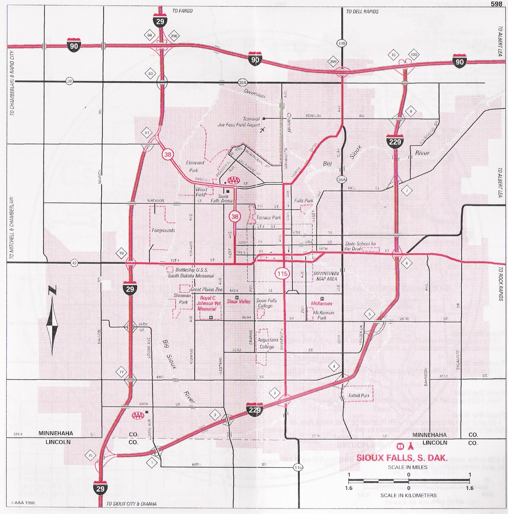
Sioux-Falls Network; Node Coordinates; Trip Table. (24 zones; 24 nodes; 76 links; toll factor=0 minutes/cent; distance factor=0 minutes/mile). Best-known link flows solution with Average Excess Cost (normalized gap) of 3.9E-15. Optimal objective function value: 42.31335287107440. A map (Reproduced by Hai Yang and Meng Qiang, Hong Kong University of Science and Technology.)
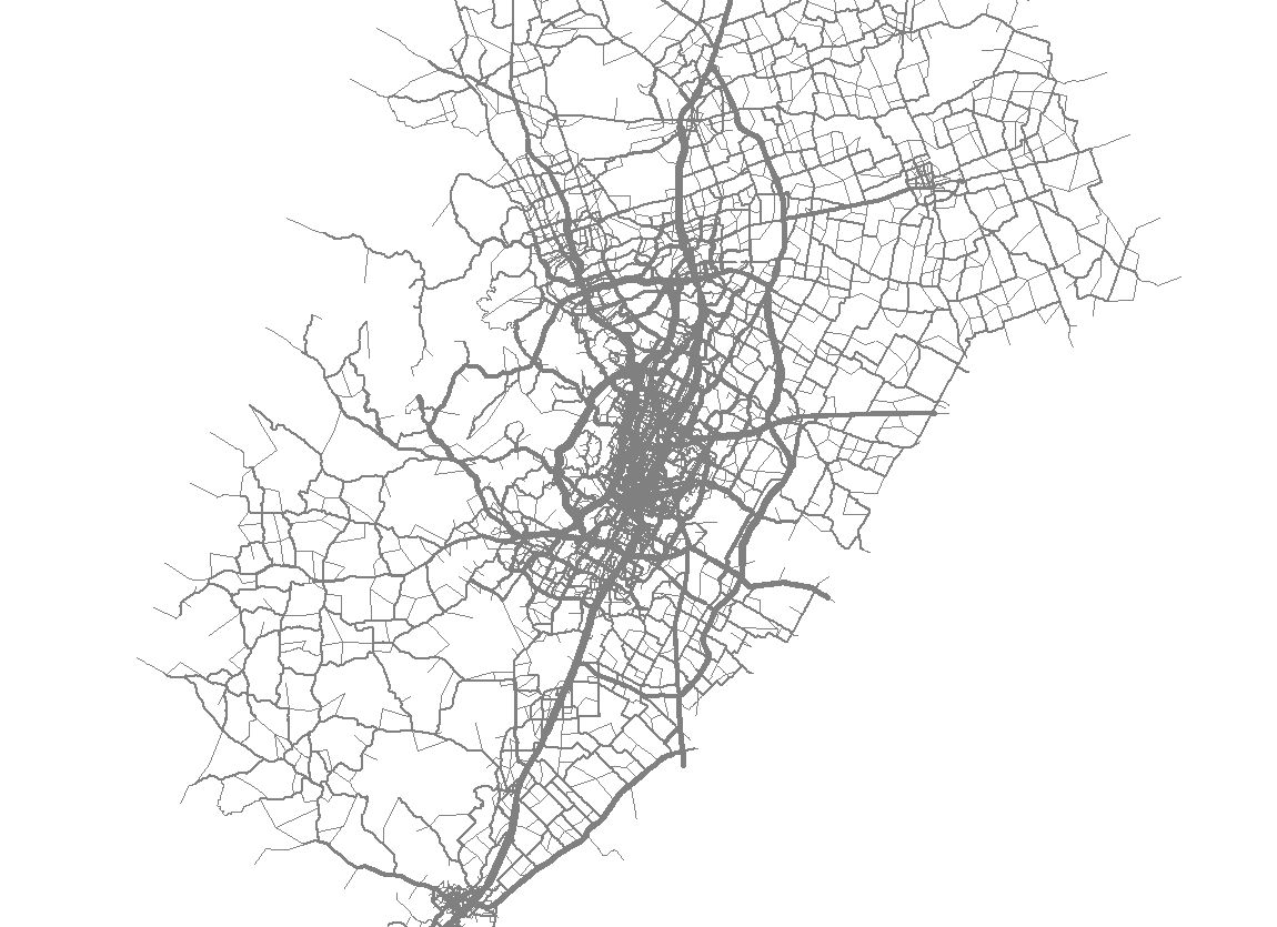
WARNING: The Sioux-Falls network is not considered as a realistic one. For comparison, see a map of the real city. However, this network was used in many publications. It is good for code debugging. It is also an opportunity to examine the data format.
All network data including the link numbers indicated on the map (but excluding node coordinates), are taken from the following paper: “An efficient approach to solving the road network equilibrium traffic assignment problem” by LeBlanc, L.J., Morlok, E.K., Pierskalla, W.P., Transportation Research Vol. 9, pp. 309-318, 1975. The links in the network file are sorted by their tail node, thus they do not follow the same order as the original publication. OD flows in the original paper (Table 1) are given in thousands of vehicles per day, with integer values up to 44. OD flows here are the values form the table multiplied by 100. They are therefore 0.1 of the original daily flows, and in that sense might be viewed as approximate hourly flows. This conversion was done to enable comparison of objective values with papers published during the 1980's and the 1990's. The units of free flow travel times are 0.01 hours, but they are often viewed as if they were minutes. Link lengths are set arbitrarily equal to free flow travel times. The parameters in the paper are given in the format of t=a+b*flow^4. The original parameter a is the free flow travel time given here. The original parameter b is equal to (free flow travel time)*B/(capacity^Power) in the format used here. In the data here the “traditional” BPR value of B=0.15 is assumed, and the given capacities are computed accordingly. Node coordinates were generated artificially to reproduce the diagram shown in the paper.
Walter Wong (kiwong@mail.nctu.edu.tw) points out that another version of the Sioux-Falls network appears in a different publication, “An algorithm for the Discrete Network,” LeBlanc, L.J., Transportation Science, Vol 9, pp 183-199, 1975. The difference between the two versions is that the free-flow travel times on links 15-19, 19-15, 15-22 and 22-15 are 4 instead of 3, and the free-flow travel time on links 10-16 and 16-10 are 5 instead of 4.
Andrew Koh (atmkoh@yahoo.co.uk) reports that a third version of the Sioux-Falls network has appeared in “Equilibrium Decomposed Optimization: A Heuristic for the Continuous Equilibrium Network Design Problem,” Suwansirikul, C., Friesz, T.L., Tobin, R.L., Transportation Science, Vol. 21(4), 1987, pp. 254-263. Click here for a list of differences between the two versions.
Gregor Laemmel (laemmel@vsp.tu-berlin.de) reports that the first published version of the Sioux-Falls network appears in "Development and Application of a Highway Network Design Model - Volumes 1 and 2," Morlok, E.K., Schofer, J.L., Pierskalla, Marsten, R.E., W.P., Agarwal, S.K., Stoner, J.W., Edwards, J.L., LeBlanc, L.J., and Spacek, D.T., Final Report to the Federal Highway Administration under contract number DOT-FH-11-7862, Department of Civil Engineering, Northwestern University, Evanston, Illinois, July 1973. Link lengths (in miles) are given the following file: Sioux-Falls Network, which is identical to the first version given here in all other attributes.
David Boyce (d-boyce@northwestern.edu) comments that yet another slightly different version of the Sioux Falls network appears in LeBlanc’s Ph.D. thesis. The main difference from the published paper version is that flows in the published paper are multiplied by 100, rounded in an unclear manner, and presented as integers, while flows in the thesis are in tenths.
See also the discussion about Sioux Falls variants for network design.
Enriched Sioux Falls Scenario with Dynamic and Disaggregate Demand was kindly provided by Artem Chakirov, from the Future Cities Laboratory (FCL) at the Singapore-ETH Centre for Global Environmental Sustainability (SEC). For additional details see Chakirov and Fourie (2014), available at http://www.ivt.ethz.ch/vpl/publications/reports/ab978.pdf.
An alternative dynamic version of the Sioux Falls network was prepared by Michal Nitzani, relying to some extent on information from Adam Pel.
Winnipeg Network; Trip Table. Units: need to check. (147 zones; 1052 nodes; 2836 links; toll factor=0; distance factor=0). There are various versions of the Winnipeg network; this is one of them. Any information on the different versions will be highly appreciated. In this version the “capacity” is arbitrarily set to 1, while the “B” value is in fact B/capacity^power. Best-known link flows solution with Average Excess Cost of 2.8E-15. Optimal objective function value: 827911.494629963.
Anaheim Network; Trip Table. Units: length is in feet; free flow travel time in minutes; speed in feet per minute. (38 zones; 416 nodes; 914 links; toll factor=0; distance factor=0). The Anaheim network for 1992 has been provided by Jeff Ban and Ray Jayakrishnan. Best known link flows solution with Average Excess Cost of less than 1E-15. A map of the Anaheim network has been provided by Marco Nie.
Barcelona Network; Trip Table. Units: probably minutes and km. (110 zones; 1020 nodes; 2522 links; toll factor=0; distance factor=0). In this network volume delay functions use high powers. Best-known link flows solution with Average Excess Cost of 2E-14. Optimal objective function value: 1265654.92203176.
Chicago Sketch Network; Node Coordinates; Trip Table. Units: minutes, miles and cents. (387 zones; 933 nodes; 2950 links; toll factor=0.02 minutes/cent; distance factor=0.04 minutes/mile). A fairly realistic yet aggregated representation of the Chicago region. Developed and provided by the Chicago Area Transportation Study. Node coordinates follow Illinois state plane coordinate system, in feet. The original data is known to provide low levels of congestion, not realistic for the Chicago region. For algorithm testing it is recommended to double the original trip table. Best-known link flows solution with Average Excess Cost of 2.1E-13. Optimal objective function value: 17313018.7387477. The preparation of this dataset is described in the following references:
- Eash, R.W., K.S. Chon, Y.J. Lee and D.E. Boyce (1983) Equilibrium Traffic Assignment on an Aggregated Highway Network for Sketch Planning, Transportation Research Record, 994, 30-37.
- Boyce, D.E., K.S. Chon, M.E. Ferris, Y.J. Lee, K-T. Lin and R.W. Eash (1985) Implementation and Evaluation of Combined Models of Urban Travel and Location on a Sketch Planning Network, Chicago Area Transportation Study, xii + 169 pp.
Austin network; Trip Table. Map. (7,388 zones, 7,388 nodes, 18,961 links). This 2005 dataset was kindly provided by Chi Xie
(chi.xie@mail.utexas.edu). The O-D trip file is for the morning peak-hour period.
Hong Zheng identified the following duplicate links in the Austin network: [1879, 1884]; [4079, 4080]; [4080, 4079]; [4436, 6583]; [6583, 4436]. Notice that the parameters of the duplicate links are not the same. Any reports using this network until 2012 should be assumed to rely on the network with the duplicated links. Any reports using this network from 2013 onwards should be assumed to rely on the network with the first link in each duplicated pair.
Chicago Regional Network; Node Coordinates; Trip Table. Units: minutes, miles and cents. (1,790 zones; 12,982 nodes; 39,018 links; toll factor=0.1 minutes/cent; distance factor=0.25 minutes/mile). A large-scale, detailed representation of the Chicago region. Developed and provided by the Chicago Area Transportation Study (CATS). Best-known link flows solution with Average Excess Cost of 8.3E-12. Optimal objective function value: 30792611.3864393. Reported network coding issues.
Aroon Aungsuyanon (aroon_jung@yahoo.com) studied the set of equilibrium PAS for this network under various demand levels. The results of his analysis can be found at: https://app.box.com/s/i7zvz5gyw8k5kweps90r (5,617 maps for CS=0.2); https://app.box.com/s/erhjbaoljv5094xhd9wr (11,702 maps for CS=0.1); https://app.box.com/s/vy53ly09y5wjwn08hqur (22,500 maps for CS=0.05).
Philadelphia Network (in the standard format, for the original older format click here) ; Node Coordinates; Trip Table; Tolls. Units: minutes, miles and cents. (1,525 zones; 13,389 nodes; 40,003 links; toll factor=0.055 minutes/cent; distance factor=0). A large-scale network for the Delaware Valley Region, provided by Dr. W. Thomas Walker, Manager, Office of Corridor/Systems Planning, Delaware Valley Regional Planning Commission, Philadelphia, PA, and are released with his permission. Node coordinates are given in units of 0.01 miles (i.e. divide by 100 to get the values in miles). To read more about this network click WORD or TEXT.
An additional set of networks from the Berlin area has been provided by Rolf Möhring (TU Berlin) Andreas Schulz (MIT), and Nicolas Stier-Moses (Columbia University) with the assistance of Stefan Gnutzmann (DaimlerChrysler). These networks were used, among other things, in the paper by O. Jahn, R.H. Möhring, A.S. Schulz, and N. Stier-Moses titled "System-Optimal Routing of Traffic Flows with User Constraints in Networks with Congestion" (Operations Research, 53:4, 600-616, 2005). The original format of these files is slightly different from the other networks, and it is described in the readme file included in the packet.
Hong Zheng identified the following duplicate links in the Berlin Center network: [1246, 1244]; [3644, 3643]; [7773, 7870]; [7777, 7779]; [8468, 8472]; [8472, 8468]. Notice that the parameters of the duplicate links are not the same. Any reports using this network until 2012 should be assumed to rely on the network with the duplicated links. Any reports using this network from 2013 onwards should be assumed to rely on the network with the first link in each duplicated pair.
A version of Berlin area data converted to the TNTP format has been prepared by Hillel Bar-Gera. Network properties are as follows:
|
Network name |
Number of zones |
Number of nodes |
Number of links |
|
berlin_center |
865 |
12,981 |
28,376 |
|
friedrichshain_center |
23 |
224 |
523 |
|
mitte_center |
36 |
398 |
871 |
|
mitte_prenzlauerberg _friedrichshain_center |
98 |
975 |
2,184 |
|
prenzlauerberg_center |
38 |
352 |
749 |
|
tiergarten_center |
26 |
361 |
766 |
PRISM-M Network; Node Coordinates; Trip Table; (898 zones; 14,639 nodes; 33,937 links). This model of the Birmingham City Region in England is a modified version of the Prism model, described at http://www.prism-wm.com/. Access to the dataset has been kindly provided with the assistance of Tom van Vuren (Mott MacDonald) and Klaus Noekel (PTV). Data format conversion and file preparation was performed by Jun Xie and Yu (Marco) Nie.
Two datasets from Australia were kindly provided by Michiel Bliemer (M.Bliemer@itls.usyd.edu.au). The source of these data is Veitch Lister Consultancy in Brisbane, Australia. These datasets are available both in the original (excel file) format, and in the TNTP format. The conversion to TNTP format was performed by David Rey (d.rey@unsw.edu.au).
Sydney (3,264 zones, 33,837 nodes, 75,379 links): Original format; Network; Node Coordinates; Trip Table.
Gold Coast (1,068 zones, 4,807 nodes, 11,140 links): Original format; Network; Node Coordinates; Trip Table. (This dataset was revised in January 2016 to resolve various inconsistencies in the previous version.)
Asymmetric Traffic
Assignment Problems
Winnipeg Network; Trip Table. Units: need to check. (154 zones; 1057 nodes; 2535 links; 0 turns; 275 asymmetric junctions). This is an asymmetric version of the problem. See explanation below about travel times in this network. This dataset has been kindly provided by Esteve Codina Sancho, Universitat Politècnica de Catalunya.
Terrassa Network; Trip Table. Units: need to check. (55 zones; 1609 nodes; 3264 links; 1103 turns; 177 asymmetric junctions). See explanation below about travel times in this network. This dataset has been kindly provided by Esteve Codina Sancho, Universitat Politècnica de Catalunya.
Hessen Network; Trip Table. Units: need to check. (245 zones; 4660 nodes; 6674 links; 7054 turns; 348 asymmetric junctions). See explanation below about travel times in this network. This dataset has been kindly provided by Esteve Codina Sancho, Universitat Politècnica de Catalunya.
The above three network (Winnipeg, Terrassa and Hessen) have an asymmetric cost structure proposed by Codina.
Supplementary Files
To get a simple source code that implements the Frank-Wolfe algorithm and demonstrates how to read these data formats click here Download FW. (This is NOT the source code for the OBA algorithm indicated below.)
Comment: the header file "stdafx.h" is related to the Microsoft Visual C (MSVC) compiler. On Unix and other compilers it can be simply omitted.
The high precision solutions presented here were produced by the Origin-Based Assignment (OBA) algorithm.
OBA executable for research purposes is now available from http://www.openchannelsoftware.org/projects/Origin-Based_Assignment/
This executable is a DOS shell application. There are two ways to run it:
1) From a DOS command window:
a) Place all the files in one directory, including "tap_ob.exe", the "tui" control file, and the input files.
b) Open a DOS command window (in windows press the "windows/start" button, in the "search programs and files" type "CMD").
c) Change directory (using "CD") to the directory where the files are.
d) Type "tap_ob.exe XXX.tui" where XXX is the "tui" control file.
2) Using a batch file:
a) Create a plain ascii text file named "ZZZ.bat", containing the following text: "<DIR1\>tap_ob.exe <DIR2\>XXX.tui > <DIR3\>YYY.txt"
b) In the above, indicating directories DIR1, DIR2, and DIR3 is optional. If indicated, the full path should be indicated, e.g. "C:\MyDir\TAP\SiouxFall\Test1\sft17.tui"
c) XXX should be the tui file.
d) YYY is an output file to collect all the screen printouts.
e) ZZZ can be any batch file name. If the command includes full paths, then the batch file can be placed anywhere. If the command does not include full paths, the batch file must be placed together with all other files in the same directory.
f) In windows explorer double click the batch file, and (hopefully) the code should run…
For an example of a control file for the origin-based code click here.
You will need to change the input and output directory.
You will also need to change the input file names according to the network you choose to work with.
A script to convert CUBE trip tables to OBA format has been kindly provided by Birat Pandey.
A
vbs script to convert trip tables from OBA format to
VISUM format has been kindly provided by Wolfgang
Scherr from PTV America.
Basic scripts for mapping networks with Matlab
Utilities to convert TransCad's trip table in comma-delimited format to the format listed here, and vice versa, have been kindly provided by Chi Xie (chi.xie@mail.utexas.edu):
TransCad to TNTP source code; TransCad to TNTP application; TNTP to TransCad source code; TNTP to TransCad application.
The command line for both programs is “program.exe input.txt output.txt”.
GML versions of all network files were kindly provided by Diego Luchi (diego.luchi@hush.com).
Links:
Test networks for the Asymmetric Network Equilibrium Problem
Open-source
GUI for visualizing static/dynamic traffic assignment results.
seSue is an
open source tool to aid research on static path-based Stochastic User
Equilibrium (SUE) models. It is designed to carry out experiments to analyze
the effects of (1) different path-based SUE models associated with different
underlying discrete choice models (as well as hybrid models), and (2) different
route choice set generation algorithms on the route choice probabilities and
equilibrium link flows. For additional information, contact Ugur Arikan
(ugur_arikan@sutd.edu.sg).
Comment: users have reported on problems with downloading data files using Netscape. Downloading seems to work fine with other browsers.
This site is managed by: Hillel Bar-Gera
Established: 2001
Last updated on April 12,
2016
Updates History
Explanation about <FIRST THRU
NODE>, May 17, 2007.
Add Berlin area networks, May 17, 2007.
Add reference to third version of Sioux-Falls
(Suwansirikul), May
17, 2007.
Comments on the FW code, May 17, 2007.
Add map for Anaheim, April 12, 2007.
Change Philadelphia network file to standard
format, April, 12 2007.
Change file names to uniform convention with
*.txt, April 12, 2007.
Add an example “tui“
control file for the origin-based assignment code, April 12, 2007.
Change the toll factors in the Chicago
networks, August 27, 2007. (The new toll factors are the ones originally used
in my own papers. For a certain period the toll factors indicated here were
zero, so it there may be publications reporting results with zero toll
factors.)
Add optimal OF values for different networks,
August 27, 2007.
Add link lengths from Morlok’s
report to the Sioux Falls network. November 19, 2007.
Update Berlin area networks data, and added
converted version for TNTP format. January 15, 2008.
Austin data added. January 12, 2011.
TransCad to OBA format conversion utility added. January 12, 2011.
Added explanation of the units of OD flows for
Sioux Falls. March 31, 2011.
Update of TransCad
conversion utilities by Chi Xie, including a fix of the previous utility.
September 26, 2009.
Addition on duplicate links as pointed out by
Hong Zheng, December 3, 2012.
Correction of the description of the Winnipeg
network from "154 zones; 1067 nodes; 2975 links" to "147
zones; 1052 nodes; 2836 links", pointed out by
Huayu (Cathy) Xu, February 7, 2013.
Addition of explanation about node
coordinates, and references, for the Chicago Sketch network. April 14, 2013.
Addition of the modified PRISM
network. May 5, 2013.
Addition of three asymmetric networks provided by Esteve Codina Sancho, August 4, 2013.
Add discussion on network design variants of Sioux Falls, August 30, 2013.
Add explanation about running DOS shell executables, and in particular how to use tap_ob.exe, February 27, 2014.
Add the "Enriched Sioux Falls Scenario with Dynamic and Disaggregate Demand" developed by Artem Chakirov, March 5, 2014.
Add Sydney and Gold Coast networks. April 24,
2014.
Add Sydney and Gold Coast conversion to TNTP
format. December 22, 2014.
Add links to Chicago Regional PAS maps.
December 22, 2014.
Add dynamic version of Sioux Falls by Michal
Nitzani, June 22, 2015.
Updated version of the Gold Coast network
(original format), provided by Mark Raadsen (the previous
file had corrupted node coordinates), August 25, 2015.
Added GML versions of all networks, August
25, 2015.
Link to seSue added,
January 1, 2016.
Revise Goldcoast
network, February 2, 2016.
Migration
notice, April 12, 2016.