

BEC2 observes asymmetric spin flipping transitions due to colored noise
Qualitative explanation of the results
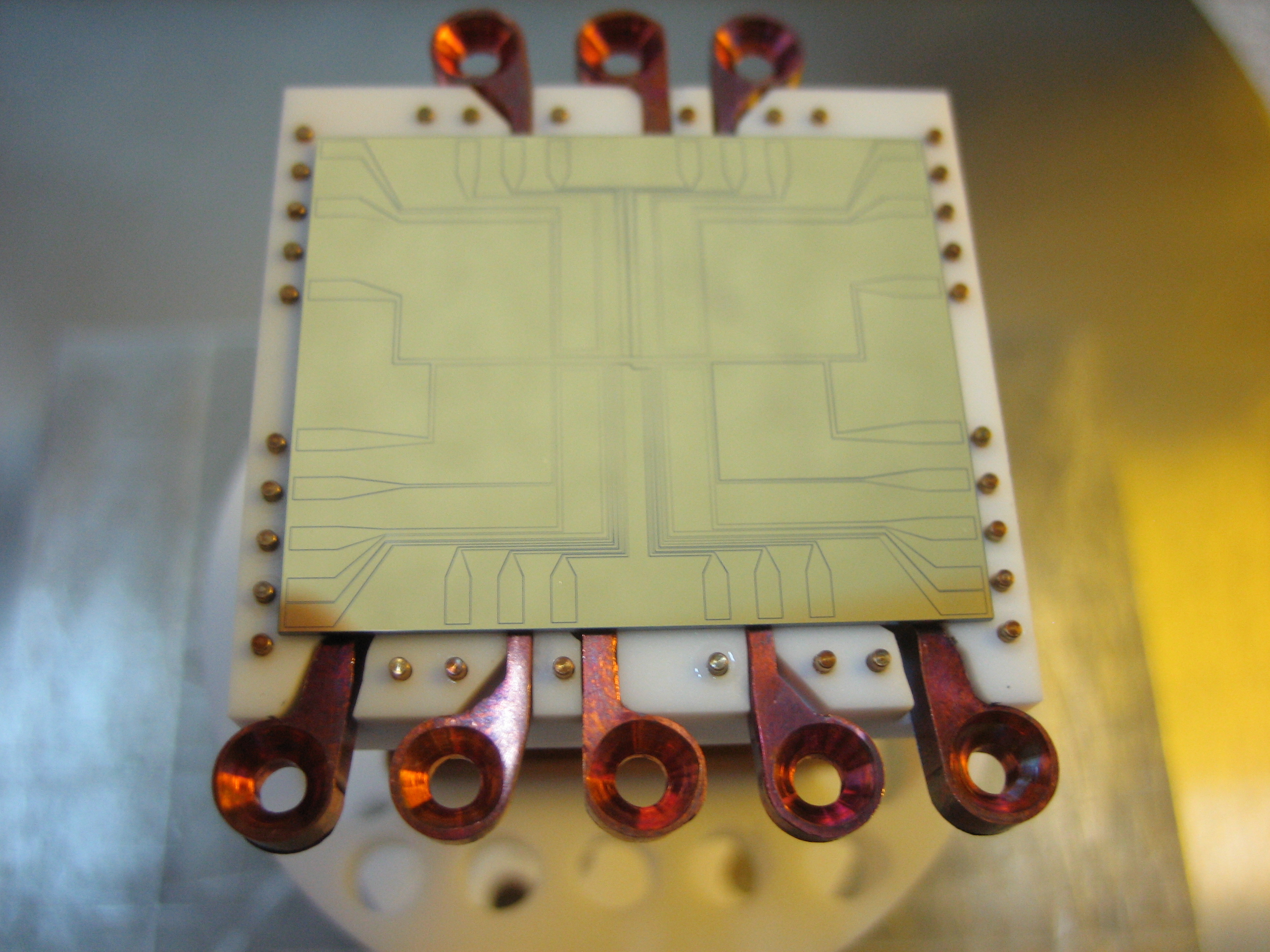
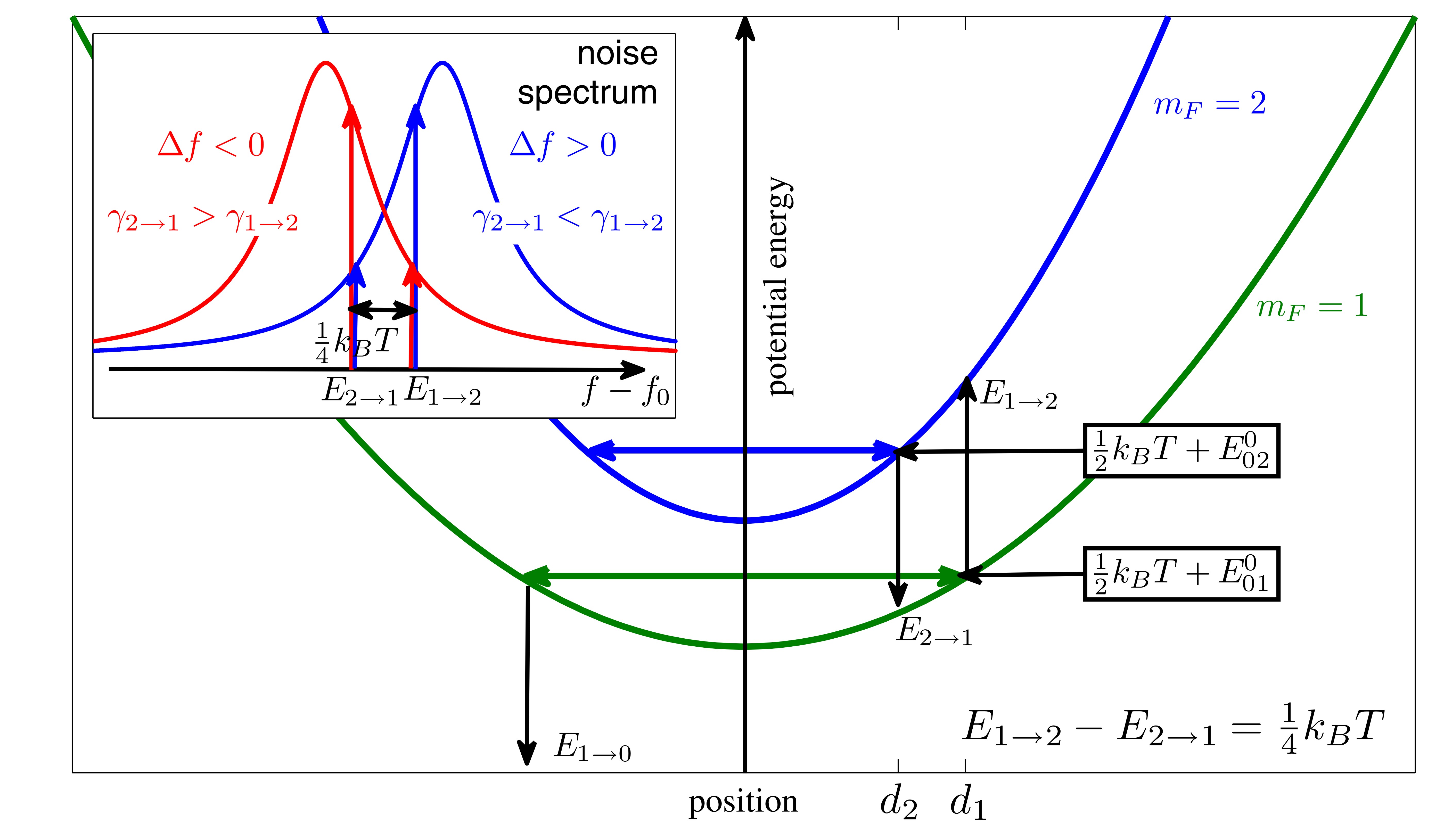
| In order to gain a qualitative understanding of the results, we present a simple semiclassical 1D model of two thermal distributions of atoms trapped in Harmonic potentials, Vj(x) = 1/2mjMω12x2, where M is the atomic mass, ω1 is the trapping frequency of the mF = 1 level and mj = mF is either 1 or 2. Each atomic distribution is represented in the figure on the right by a typical atom at an average position, di = √(kBT/mjMω12). |

Full size image |
The transition of a typical atom from mF = 2 to mF = 1 requires a photon energy E2→1 = E120 + V2(d2) − V1(d2) = E120 + 1/4kBT and reduces the energy of the atom relative to the trap bottom by 1/4kBT. A transition of a typical atom in mF = 1 to mF = 2 at d1 = √2d2 requires a photon energy E1→2 = E120 + V2(d1) − V1(d1) = E120 + 1/2kBT and increases the energy of the atom by 1/2kBT.
The relative transition rates depend on the number of photons with the two energies E1→2 > E2→1 . If the noise intensity increases with frequency in a wide enough band (∼ kBT) around f = E120/h (see blue arrows in the inset, Δf > 0), the transition 1 → 2 is preferred and the population of mF = 1 is depleted, as in the plateau on the right-hand side of the right figure below. If, by contrast, the intensity decreases in this band (see red arrows in the inset above, Δf < 0), the transition 2 → 1 is preferred and the population of mF = 1 becomes dominant, as in the plateau on the left-hand side.
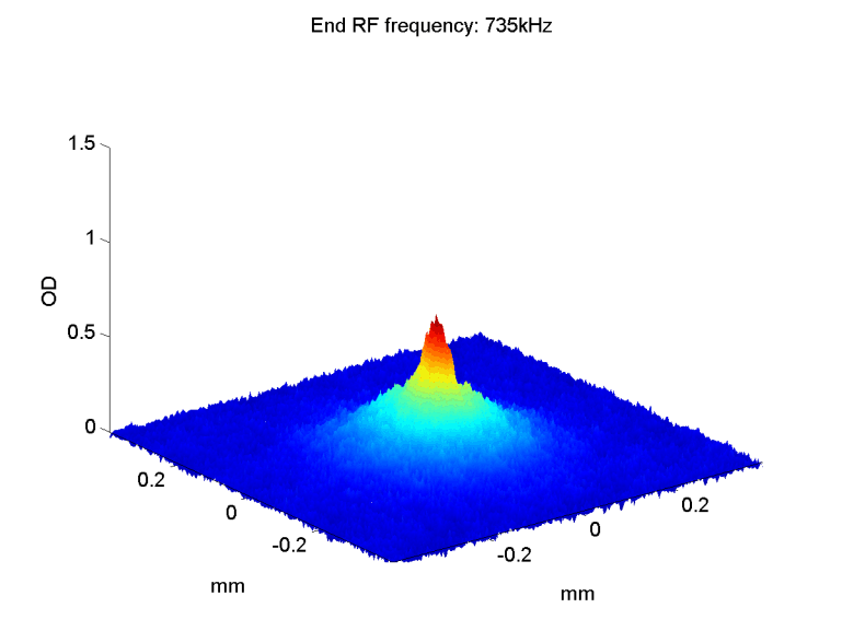
Due to these effects, even when the noise intensity decreases by a few orders of magnitude (side peaks of the noise, inset below), the atoms are still sensitive to the details of the spectrum, as can be seen in the right figure below. This may prove to be a useful tool for characterizing noise features. Note also that the temperature determines the width of the spectral region the cloud samples, hence colder clouds are more sensitive to the fine details of the noise (e.g. 1 μK gives a resolution of 20 kHz). This effect is most noticeable at Δf ≈ 0.7MHz (right figure below) where the temperature band becomes much wider.
The results
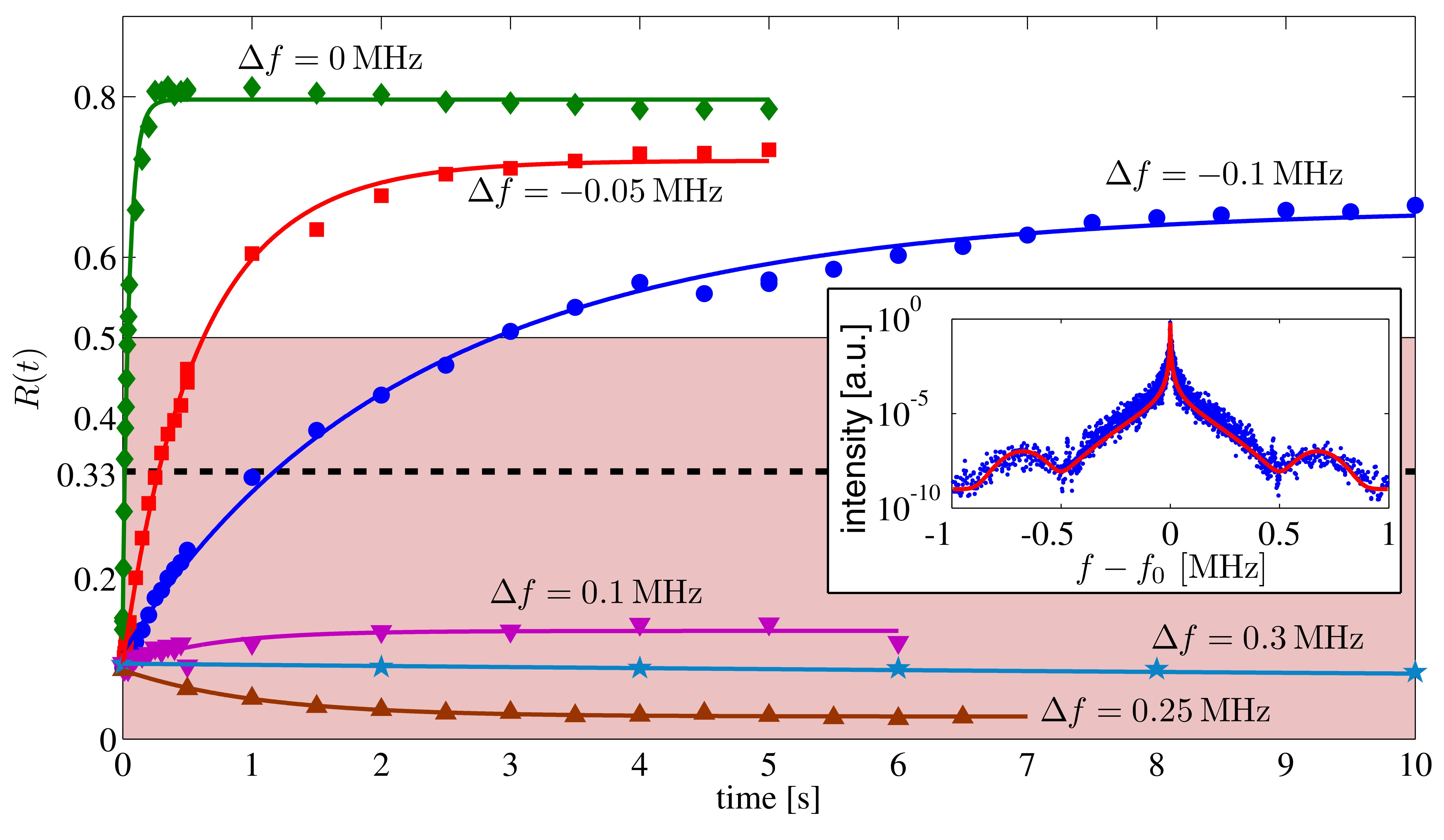
The left figure below presents the ratio R(t) = N1/(N1 + N2) as a function of the time for which the noise is applied, for different detuning Δf between the noise peak frequency f0 and the Zeeman splitting E120/h of the two trapped levels at the magnetic field minimum. The inset presents the spectrum of the noise we introduce. One may observe a large difference in the evolution of R(t) between red- and blue-detuned noise. When the noise is red-detuned (Δf < 0), the mF = 1 level is populated while when the noise is blue-detuned (Δf > 0) the mF = 1 level is depleted. The solid curves are fits to the empirical form R(t) = R∞ + (R0 − R∞)exp(−γt), which represents an exponential convergence from the initial value R0 ≡ R(t = 0) to an asymptotic value R∞ ≡ R(t → ∞).
These results show that the relative transition rates between the levels strongly depend on the detuning of the noise and significantly differ from the expected rates in the case of white noise (dashed line) or a model where the external degrees of freedom are decoupled from the transition dynamics (0 ≤ R ≤ 1/2 band).
In the right figure we plot the measured value of R∞ for different values of the center frequency of the applied noise. The band and the three curves represent the theoretical prediction for R∞, as qualitatively described above.

Full size image |

Full size image |
More details on the experiment and the quantitative explanation are explained in our paper.